Northwinds Business Analysis - More that a Professional Salesman, I'm a Business Consultant

For the Northwinds business analysis project, I worked with the Northwind database, which is a fictious database for a consumer products company that has offices in the Seattle, Washington, USA and London, British Isles. After analyzing the database, I’ll provide insight and recommendations to the Northwinds’ ‘Stakeholders’.

Data will be explored that will reveal business related questions and each question will be answered using Hypothesis Testing. Throughout this process, valuable knowledge will be gained and based on the results of the tests, conculsions and recommendations will be offered.

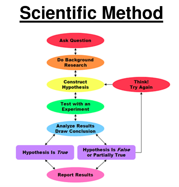
The Scientific Method (shown below) will be used as a guide.

*STEP 1: ask business related questions, such as:

Questions about the company:

- How long has Northwinds been in operation?
- Where are they based?
- What do they sell and in what categories?
- How is the sales team configured?

Questions about their customers:

- Who are their customers and where are they located?
- How much do they buy and at what frequency, quantity, and revenue?

*STEP 2: Background Research, (aka Exploratory Data Analysis) to further develop business insight and start to formulate Hypothesis Test Questions:

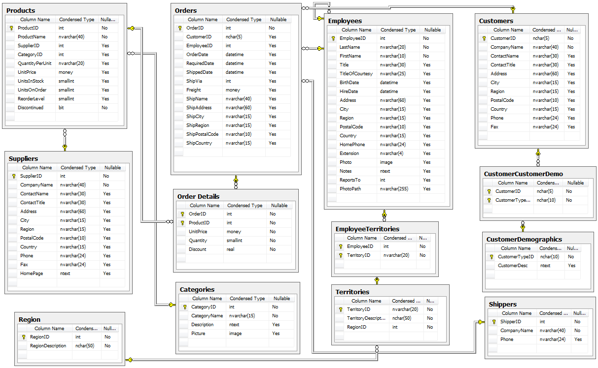
Information for Northwinds is stored in their database in tables. Here is their ERD, (Entity Relationship Diagram).

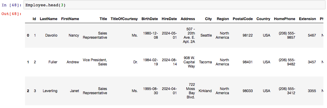
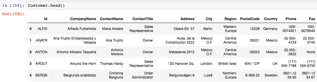
Here’s an example of the pandas query to store the table in a pandas table, along with the first few lines of the “Employee” Table.

Employee=pd.read_sql_query(‘'’SELECT * FROM Employee’’‘,conn)

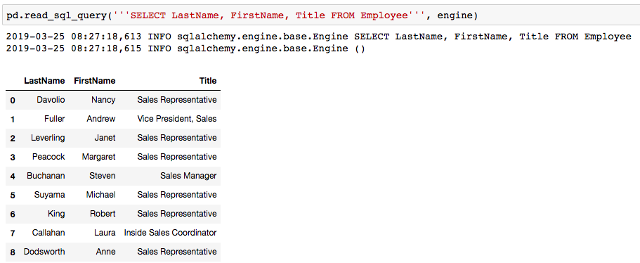
Here’s an example of an SQL Query to extract information from the same “Employee” Table.

Throughout the EDA process, I found that it was easier to work with Pandas table merges and queries instead of SQL. This was a major decision point for me.

I am comfortable using both and did so in this project. Northwinds is a relatively small database, so my computer had the memory to store each table as a Pandas DataFrame. Had the database been larger, than it would have required too much memory to store each individual Table. At that point, I would have used more SQL queries. However, for this project, each individual table name was stored using Pandas.

The most important EDA discoveries were……

EDA on the “Territory”, “EmployeeTable”, and “Region” tables and then the “Customer” Table, it’s found that the former tables did not provide the most useful information. I found that it was best to group Customers and Orders using the “Region” and “Country” columns in the ‘Customer’ table.

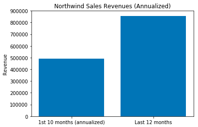
Northwinds has orders dating from July 4th, 2012 to May 6th, 2014. My next major decision point, was how to segment the sales data. I’ve sent much of my career in sales and typically make presentations that compare sales data on an annual basis. The Northwind Sales are over a 22 month period, so I decided to segment sales as follows: .

1st segment is the first 10 months.

July 4th, 2012 to May 6th, 2013
The 10 month period was the period remaining after having to segment the “Last 12 months”.
First 10 months are annualized (Sales / 10 months * 12 months)
281 Orders (745 OrderDetails) worth 408,908( 490,690 annualized)

2nd segment is the last 12 months.

May 7, 2013 to May 6, 2014
Stakeholders (Senior Management) look at data on a year to year basis
549 Orders (1059 Order Details) worth $856,885

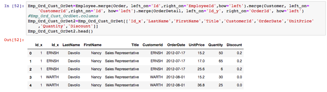
Next, I merged to Customer, Order, OrderDetail, and Employee Tables to perform more EDA. Below is the code for the merge and the resulting table.

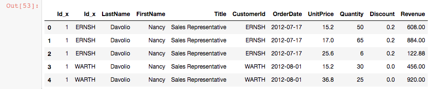
And then I made a “Revenue” column by multiplying the “Quantity”, “UnitPrice”, and “Discount” columns.

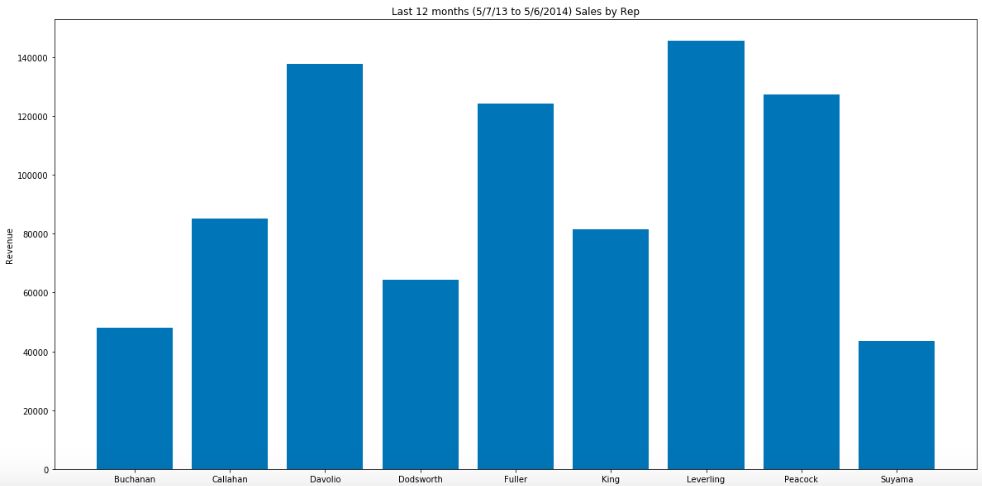
Here is the Total Revenue for the last 12 months for each salesperson. I used the Pandas ‘groupby’ method to ‘sum’ the Total Revenue by salesperson, which is summarized below.

Then I started looking at Hire Date, Number of Territories, Average Order Size by Customer by Salesperson, and Average Revenue by Customer by Salesperson. With further EDA, I found that these predictors were faulty for the following reasons:

-Hire Dates show values that are in the future and therefore not accurate.

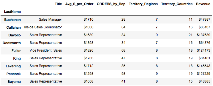
-When I looked at the locations of the customers and salesperson assigned to each order, I discovered that all salespeople were not limited by geographical boundaries when selling to customers. There are 9 Salespeople based in 2 locations: Seattle, WA and London selling into a total of 9 Regions and 21 Countries. They all sell to customers in multiple countries and regions. It appears that each salesperson sells into most of the countries and regions. There are no sales territory boundaries.

-Therefore, “Number of Territories” nor “Average Revenue by Customer by Salesperson” were not good predictors. Therefore, “Average Revenues per Order “per Salesperson and “Number Orders per Salesperson” will be tested.

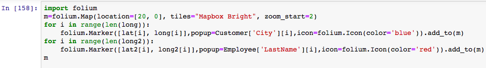
Next, it was important to get a Geographic Overview of the locations of Northwind’s customers and salespeople. I used geopy and folium to produce the map below.

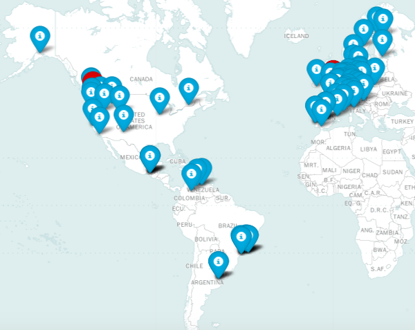
Visually, the map shows a concentration of customers in the US Pacific Northwest and in Western Europe. This makes sense, since the salespeople are physically located in Seattle, WA and London.

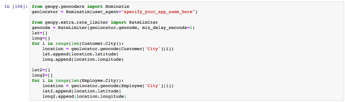
Here’s the code to get the longitute and latitude of each customer and employee city:

Here’s the code to “mark” each longitude and latitude on a FOLIUM map:

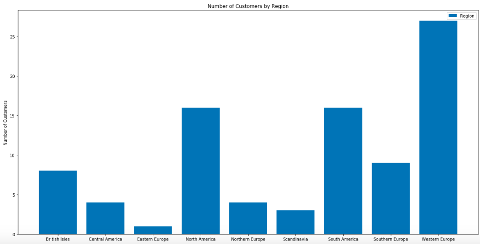
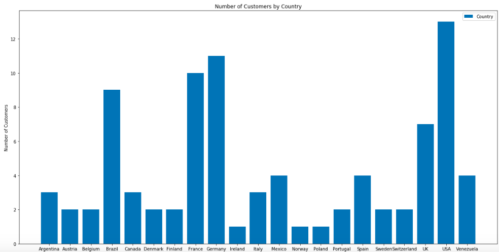
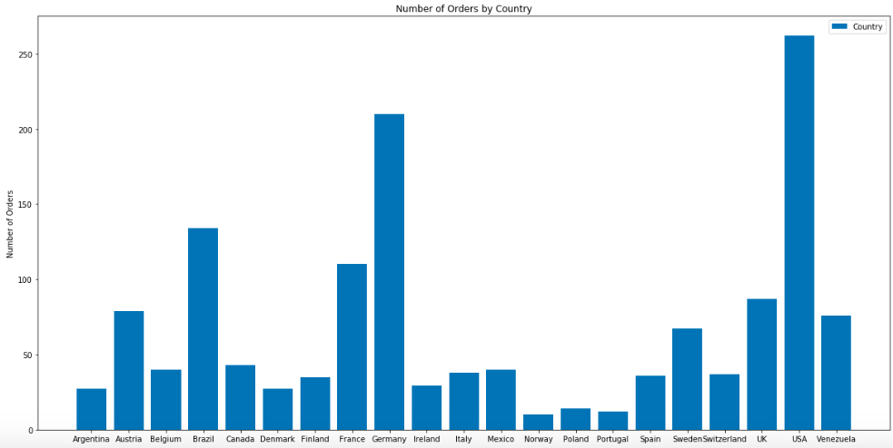
Below are bar charts that visualize the number of customers by ‘region’ and by ‘country’.

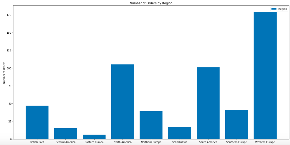
And here are the number of orders by ‘region’ and ‘country’.

The EDA was very informative and several important questions were ‘revealed’ that will provide relevant information to Northwind’s stakeholders. Here are the questions:

DO DISCOUNTS HAVE A STATISTICALLY SIGNIFICANT AFFECT ON THE NUMBER OF PRODUCTS CUSTOMERS ORDER? IF SO, AT WHAT LEVEL(S) OF DISCOUNT?
WHICH PRODUCTS OF CATEGORIES SELL BETTER WITH A DISCOUNT?
IS THERE A METHOD TO IDENTIFY THE TOP PERFORMING SALESPEOPLE AND COMPENSATE THEM ACCORDINGLY?
DO WE GROW OUR BUSINESS BY FOCUSING OUR EFFORTS ON UNDERPERFORMING GEOGRAPHIC AREAS? OR DO WE EXPAND INTO OVERPERMING AREAS?

STEP 3: HYPOTHESIS QUESTIONS: The next step to prove(disprove) hypothesis questions using statistical test.

QUESTION 1: DO DISCOUNTS HAVE A STATISTICALLY SIGNIFICANT AFFECT ON THE NUMBER OF PRODUCTS CUSTOMERS ORDER? IF SO, AT WHAT LEVEL(S) OF DISCOUNT?

-NULL HYPOTHESES: The average quantity of product sold in the same for orders with or without a discount.

-ALTERNATIVE HYPOTHESIS: The average quantity of product sold with a discount is higher than product sold without a discount.

-ONE-TAIL TEST and ALPHA = .05

This will require a one-tail test, because the business is interested if a discount will statistically increase sales. If the null hypothesis is rejected, then there is a statistically significant increase in the quantity of products sold with discounts.

To test the hypothesis, we will be using the table ‘OrderDetails’ and looking at the columns ‘Quantity’ and ‘Discount’. Below we can see that there are no NaN nor missing values in either column. Also, ‘Quantity’ ranges from 1 to 130 and ‘Discount’ ranges form 0 to .25.

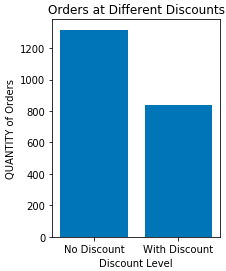
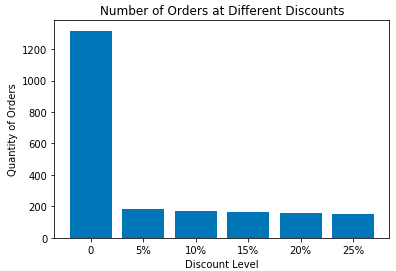
Below is a summary of TOTAL NUMBER of orders written in the 22 months that Northwinds has been in operation.

2155 order “line items” written in 22 months
1317 orders were sold with NO discount, 838 sold with discount
Discounts ranged from 5% to 25%

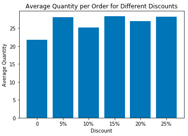
Next, the graphs below will show the AVERAGE order size at different discount levels:

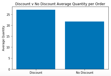
The Discounted Orders Mean and Median are 27.1 and 20.0, respectively. The Non-Discounted Orders Mean and Median are 21.7, and 18.0, respectively

Now a Ttest will be run on the 2 different samples to see if they are statistically from the same set. A 2 Sample Ttest is used because we have two samples.

The above test is a two-sided ttest, so we take pvalue/2 for a one-sided test. Our resulting pvalue is still < our alpha (.05), so this is an indication that we will REJECT THE NULL HYPOTHESIS.

Next, let’s calculate Effect Size for the Discount v Non-Discount using Cohen’s D. It’s the most commonly used measure of Effect Size. I’ll use it to measure the difference between Discount and Non-Discount. A large value will represent a significant difference.

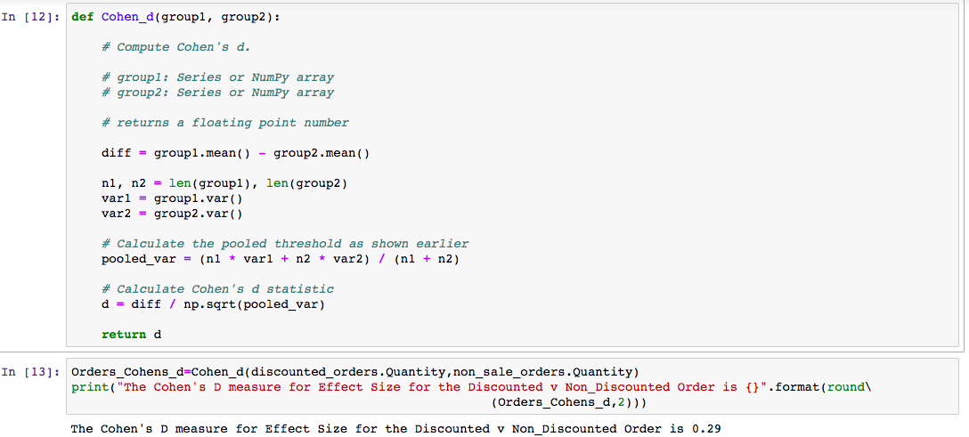
The basic formula to calculate Cohen’s d is: effect size (difference of means) / pooled standard deviation

Interpreting Cohen’s D:

-Small effect = 0.2
-Medium Effect = 0.5
-Large Effect = 0.8

Therefore, our result is 2.9, so our samples have a relatively small Effect Size.

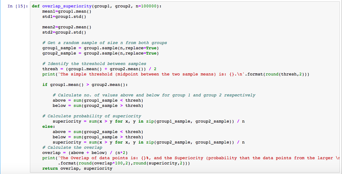
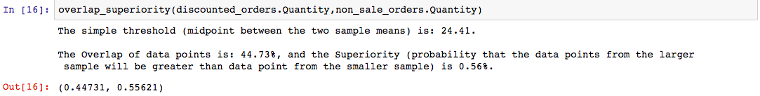
Next, there is another common way to express the difference between distributions: Overlap and Superiority.

“Overlap” (or misclassification rate), and “probability of superiority” have two good properties:

-As probabilities, they don’t depend on units of measure, so they are comparable between studies.
-They are expressed in percentages, so we have a sense of what practical effect the difference makes. Superiority is the probability that a randomly data point from the larger sample will be greater than a randomly chosen data point from the smaller sample. (ex: If there’s no overlap, then superiority would be 100%).

Below are functions that compute overlap and probability of superiority, along with our results.

CONCLUSION: Since the p-value for the Ttest is <.05, the NULL HYPTOTHESIS IS REJECTED. It is statistical significant that discounted orders are NOT from the same sample as non-discounted orders. Therefore, DISCOUNTING DOES INCREASE THE QUANTITY OF ORDERS.

Next, I’ll test whether the discount LEVEL has an affect on the quantity size of the order.

Visually, there’s not a difference between the average size of the orders at the different discount levels. I’ll use a TWO-SIDED ANOVA TEST to check. This will test the overall variance as compared to the variance within each category. A pvalue above our alpha (.05) indicates that all the categories (of discounts) are statistically similiar.

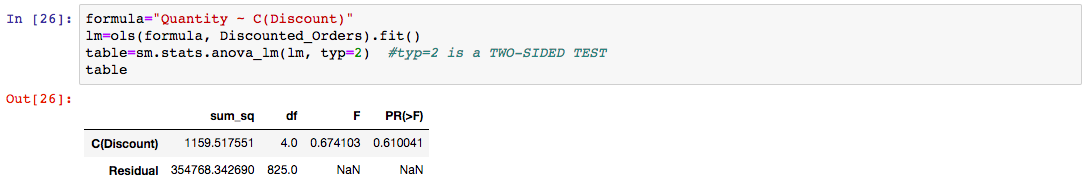
The p-value (PR>F) of our categorical “Discount” variable is .61. Since this value is >.05, we FAIL TO REJECT the null hypothesis. CONCLUSION: This suggests that the average quantity per order is not statistically significant at different discount levels. BUSINESS INSIGHT: a low level of discount should be used to maintain profit margin since it produces the same size orders.

QUESTION 2: WHICH PRODUCT CATEGORY(S) SELL BETTER WITH A DISCOUNT?

-NULL HYPOTHESIS: All products sell the same with a discount.

-ALTERNATIVE HYPOTHESIS: Products categories sell at higher (or lower) quantity when offered at a discount.

-TWO-SIDED TEST and ALPHA = .05

To test our hythosis, we will need data from more than one table, so we’ll need to join tables. First, the ‘Product’ table will be joined to the ‘OrderDetail’ as ‘Prod_Ord_Detail’; and then merge with the ‘Categories’ table.

Since we want to test the ‘Discount’ and ‘Category’ on ‘Quantity’ for ‘CategoryName’, we will use ANOVA to test the hypothesis. The ANOVA Test is comparing the variance of the “CategoryName” & “Discount” to the overall variance.

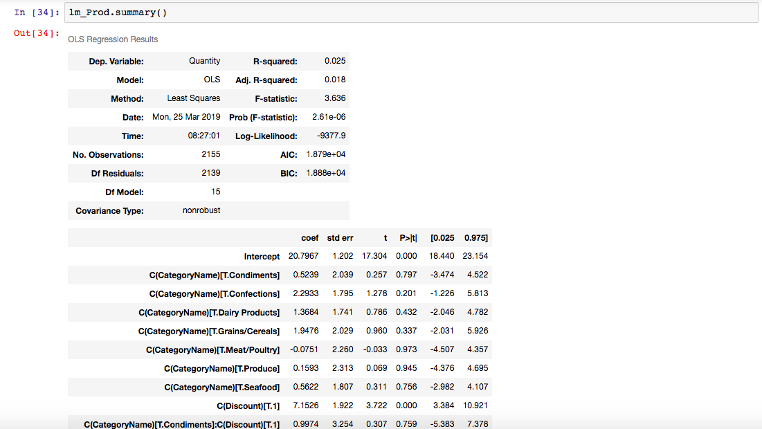
From the above table, we can see that the interaction of ‘CategoryName’ and ‘Discount’ has a p-value < .05. So, we REJECT THE NULL HYPOTHESIS. There is a stastical difference in quantity of product ordered by atleast one of the Category when a discount is applied. THEREFORE, the Different Categories react differently to being sold at a discount.

I’ll use an “interaction” plot to visualize the different category sales at “no discount” and “discount”. Here’s the code and the graph.

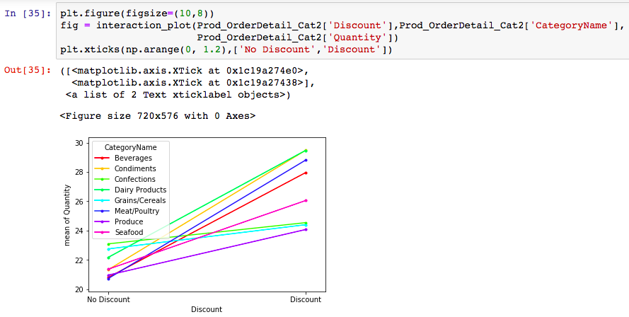
In the above visualization, lines that have similar slopes have similar interactions between “CategoryName” & “Discount” ‘Confections’ and ‘Grain/Cerels’ have visually DIFFERENT slopes than the other 6 categories. Visually, these 2 categories are SIGNIFICANT. And for Confections, this is proven by the ANOVA test.

CONCLUSION: Our findings signify that there is sufficent evident that Confections (and possibly ‘Grains/Cereals) do NOT benefit from discounting. Conversely, Meat/Poultry, Condiments, and Beverages DO benefit from selling at a discount.

The higher the slope, the more reactive to a discount. Flat line categories are unaffected by discounts.

OVERALL DISCOUNT CONCLUSIONS:

Discounts increase the average size of the order from 21.7 to 27.1
The size of the discount does not matter.
Northwinds should Discount: Meat/Poultry, Condiments, Beveragesto increase order size.
There’s no need to discount Confections nor Grains/Cereals.

QUESTION 3: IS THERE A METHOD TO IDENTIFY THE TOP PERFORMING SALESPEOPLE AND COMPENSATE THEM ACCORDINGLY?

NULL HYPTOHESES: All Salespeople produce the same.

ALTERNATIVE HYPOTHESES: Salespeople generate are different in their production.

ALPHA = 0.05 and this is a TWO-SIDED Ttest.

Next, I’ll analyze the Northwinds Sales Team. First, I’ll identify the names of the salespeople and the number & names of their territories. The goal is to identify the top performers and their attributes. These attributes can then be used to incentivize all salespeople, so that the goals of the salespeople are aligned with the goals of the company.

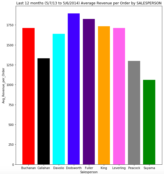
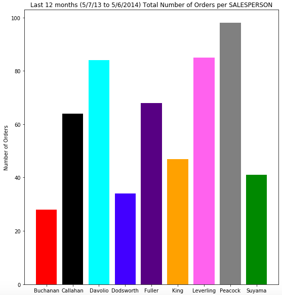
Below are 3 graphs that show the Total Revenue by Salesperson, along with their Number of Orders and Average Revenue per Order.

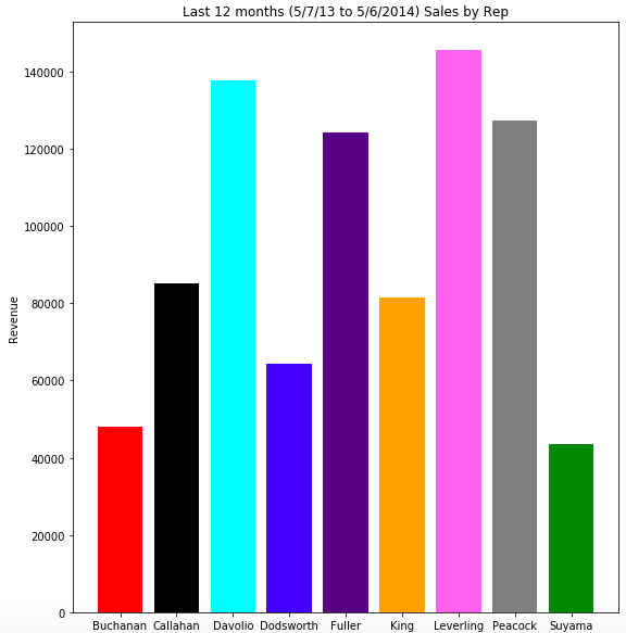
-Leverling is the Salesperson with the highest total revenue, followed by Davolio. Suyama had the lowest total Revenue.
-Peacock has the highest Total Number of Customers, followed by Davolio. Buchanan has the smallest number of Customers.
-Leverling has the highest average revenue per customer, followed by King. Suyama has the lowest.
-Callahan has the highest average number of orders per customer, followed closely by Leverling and Peacock. Suyama has the lowest.
-Peacock has the highest number of total number of orders, followed by Leverling and Davolio. Buchanan has the lowest.
-Dodsworth has the highest average revenue per order, followed by Fuller. Suyama has the lowest.

The “Revenue by Salesperson” and “Number of Orders by Salesperson” histograms seem to lend evidence to REJECT the Null Hypothesis. There appears to be difference in the each Salesperson’s Revenue.

First, let’s calculate the total orders for each salesperson in the last 12 months. Then, I’ll run an Ordinary Least Square model (OLS) on Salespeople with the following predictors: Average Revenues per Order and Number of Orders by Salesperson to see which predictor has the most influence on Revenue. Then, I’ll dig deeper into that predictor to see if there’s a difference in Sales Rep Performance.

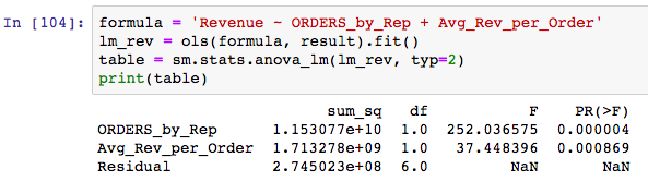
It appears that Avg_Revenue_per_Order (pvalue < .05) and TOT_Num_ORDERS_by_Rep (pvalue < .05) are influential in PREDICTING THE REVENUE of each Salesperson. Orders by Rep is the most influencial. However, this DOES NOT prove or disprove our null hypothesis. Our null hypothesis is to see if there’s a difference in salesperson revenue performance.

Let’s dig deeper and run an ANOVA test to compare Avg_Revenue_per_Order to see if there’s a statistical difference in Salesperson Performance. This will answer the question of whether the average revenue per order varies between different salespeople and assesses the degree of variation between multiple samples, where each sample is a different salesperson.

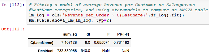
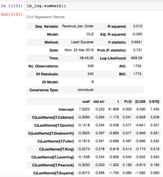
CONCLUSION: The pvalue is greater that alpha (.05), so we FAIL TO REJECT the null hypothesis. Therefore, we conclude that each salesperson is similar in terms of Average Revenues per Order.

BUSINESS INSIGHT: There is a noticeable difference in Revenue produced by each salesperson. Number of Orders and Revenue per order are strong predictors of Salesperson Total Revenue, with Number of Orders being the most influencial. The significant difference in Salesperson Total Revenue is not attributed to “Average Revenue per Order.” Therefore, the significant difference can be attributed to the number of orders. So, the Salesperson should devote his/her time to increasing their number of orders..

QUESTION 4 (YES!!…..FINAL QUESTION): Do we grow Northwinds’ business by focusing efforts on underperforming regions? Or do we expand into other Regions?

NULL HYPOTHESES: All geographical areas (Region and/or Country) are equal.

ALTERNATIVE HYPOTHESIS: Areas are different and there’s an opportunity to grow in existing territories and/or expand into others.

TWO-TAILED TEST & ALPHA = .05

First, we will start by mapping our current customers and orders, of which, there are 88 and 540, respectively. It was important to revisit the Geographic Overview that was developed in the EDA.

Visually, the map shows a concentration of customers in the US Pacific Northwest and in Western Europe. This makes sense, since the salespeople are physically located in Seattle, WA and London.

Concentration of Customers in:

Regions of W. Europe (27), N.America (16), S. America(16)
Countries of USA (13), Germany (11, France(10)

Orders in:

Regions of W. Europe (179), N. America (103)
Countries of USA (100), Germany (80), Brazil (51)

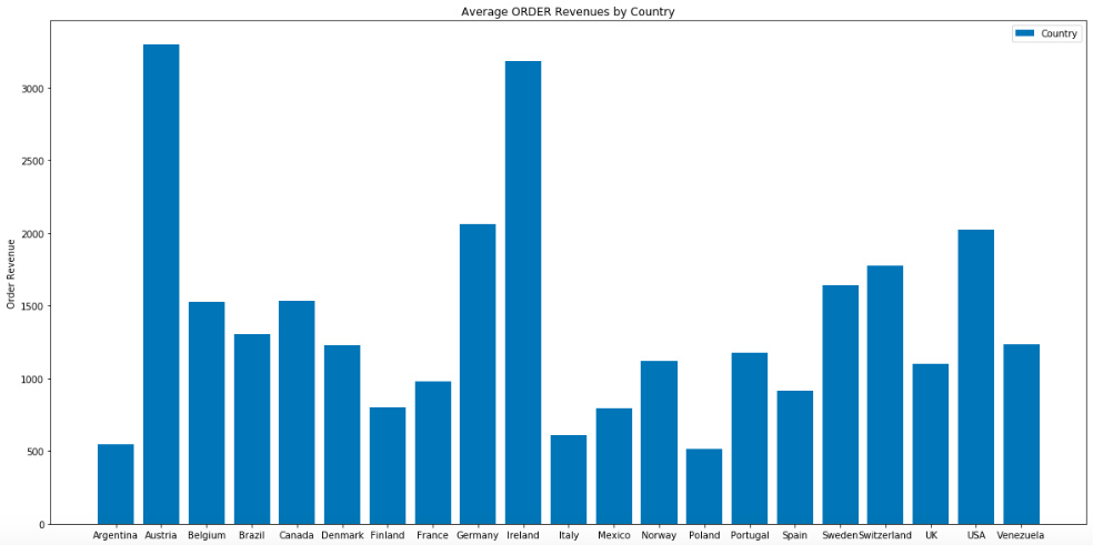
In our EDA, we discovered that the best method to differentiate geographic areas was by “Average Revenue per Order by Country.” Here are the Average Orders per Country in the Last 12 Months (5/7/13 to 5/6/14).

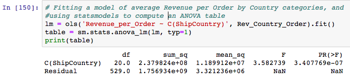
The pvalue is <.05 for Austria, so we REJECT the NULL HYPOTHESIS that the Average Customer Revenues are the same by Country.

Here is the code for Tukey test and it’s output. I used it because it’s output displayed which specific countries were different.

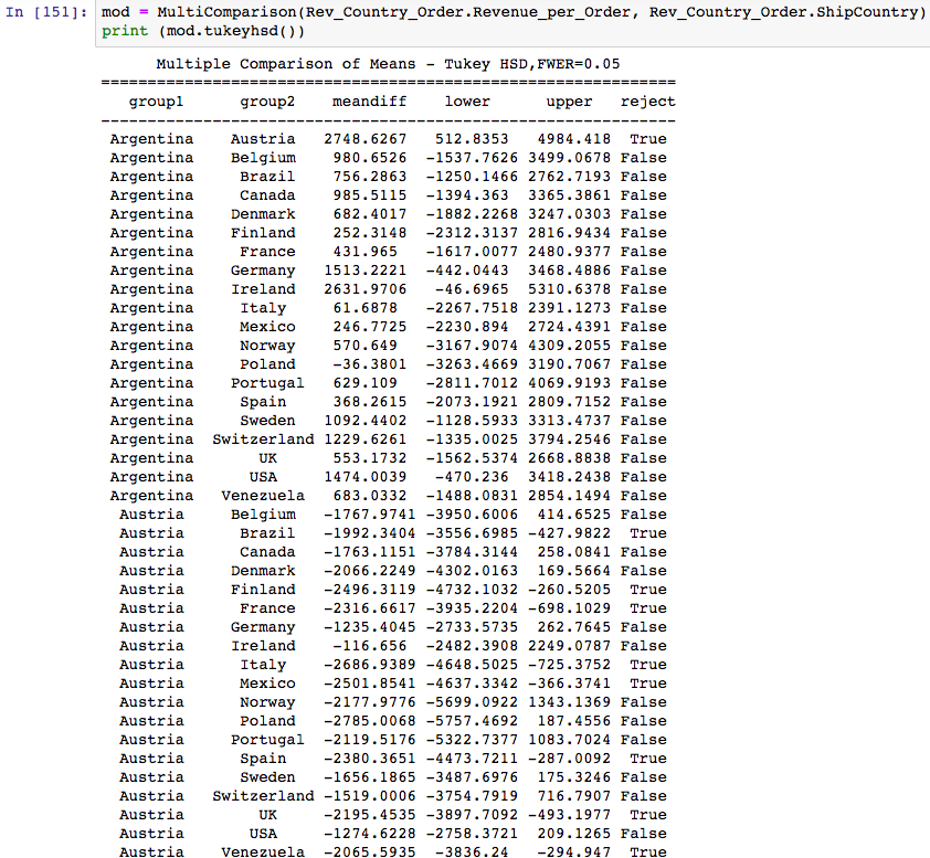
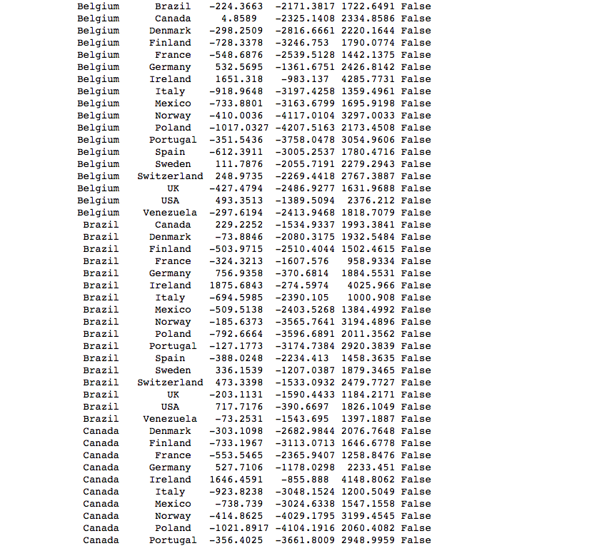
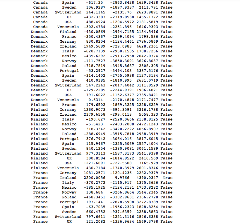
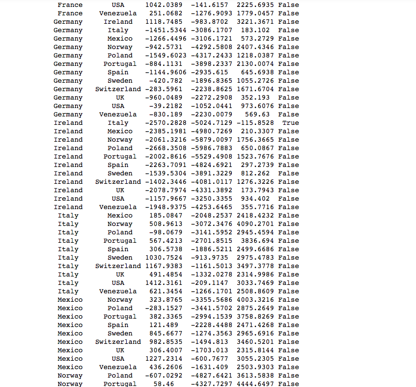
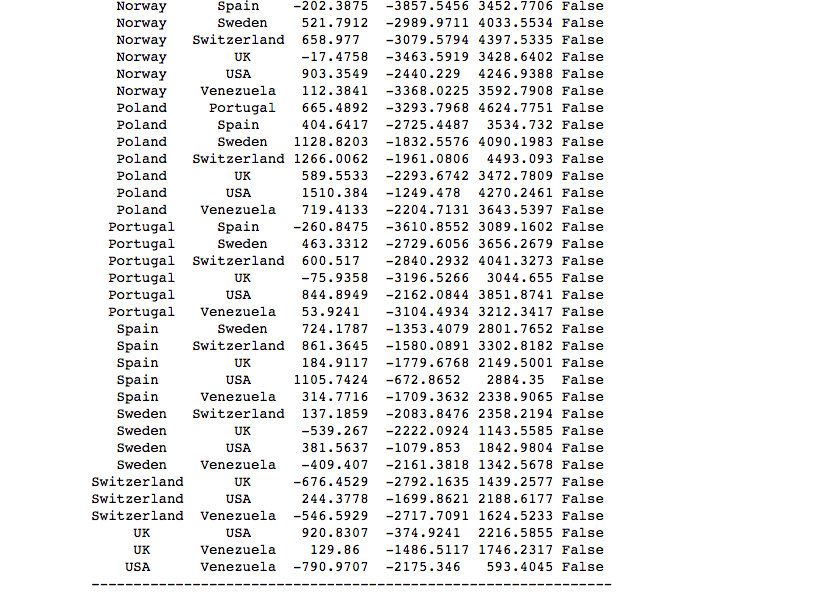
The Tukey Pairwise test shows that, given an alpha=.05, that the following pairs of Countries have statistically significant “Average Revenue per Orders”. Countries listed are statistically different than 2 or more other countries.

Austria is different from: Argentina, Brazil, Finland, France, Italy, Mexico, Spain, UK, Venezuela
Ireland is different from: France, Italy

CONCLUSION: I REJECT THE NULL HYPOTHESIS that all countries are the same in terms of “REVENUE PER ORDER.

Austria and Ireland are statiscally different than 2 or more other countries to the right (greater) of the mean.
France and Italy are statiscally different than 2 or more other countries to the left (less) of the mean.

BUSINESS INSIGHT:

There’s an opportunity to increase “REVENUE PER ORDER” with NEW customers in Austria and Ireland.
There’s an opportunity to increase “REVENUE PER ORDER” with CURRENT customers in France and Italy.

EXECUTIVE SUMMARY:

USE of DISCOUNTS:

Discounts increase the average size of the order from 21.7 to 27.1
The size of the discount does not matter.
Northwinds should Discount: Meat/Poultry, Condiments, Beveragesto increase order size.
There’s no need to discount Confections nor Grains/Cereals.

SALES TEAM INSIGHT: There is a noticeable difference in Revenue produced by each salesperson. “Number of Orders” and “Revenue per Order” are strong predictors of “Total Revenue by Salesperson”, with Number of Orders being the most influencial. The significant difference in Salesperson Total Revenue is not attributed to “Average Revenue per Order.” Therefore, the significant difference can be attributed to the number of orders. So, the Salesperson should devote his/her time to increasing their individual number of orders.

GEOGRAPHIC AREA OPPORTUNITIES: There’s an opportunity to increase “REVENUE PER ORDER” with NEW customers in Austria & Ireland (& possibly Germany and USA). There’s an opportunity to increase “REVENUE PER ORDER” with CURRENT customers in France and Italy.