ARE THERE OUTLIERS in a Model? How are they identified? How are they dealt with? How do they affect the predicability of the model? In a recent project to identify the best predictors for Home Prices in Kings County, Washington, this was the question.
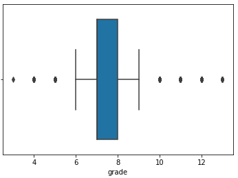
I used 2 methods to identify outliers. The first was boxplots to visualize them (ex: sns.boxplot(x=kc_house[‘grade’])). Outliers are outside the ‘whisker’ lines.
The second method is to use Interquartile Ranges (IQR). IQR is the width of the box in the box-and-whisker plot. That is, IQR = Q3 – Q1 . The IQR is used as a measure of how spread-out the values are. Q3 is the 75% percentile and Q1 is the 25% percentile. Statistics assumes that your data is normally distributed around a central value. The IQR tells how spread out the “middle” values are and it is used to identify outliers. Outliers are “too far” from the median.

The IQR is the length of the box in your box-and-whisker plot. An outlier is any value that lies more than one and a half (IQR x 1.5) times the length of the box from either end of the box. Much of the research states that outliers are identified using IQR x 1.5 However, one source used IQR x 3. I like this conservative approach in removing data. In the table above:
- Q3 (75% percentile) = 8
- Q1 (25% percentile) = 7
- IQR = 1
Therefore, using (IQR x 1.5), outliers are < 5.5 and > 9.5. However, using IQR x 3, outliers are < 5 and > 11. In my model, I choose to be conservative in removing data, so I’ll use IQR x 3. This only removed 102 rows of data from 21,587 rows.
HOW DO OUTLIERS AFFECT THE MODEL?
Initially, I did not drop outliers. After completing an initial model, I decided to circle back and analyze removing outliers to improve the predictability of the model. I found that my Rsquared with the outliers included was .65. And when I removed the outliers, the Rsquared dropped to .62. So, there was an argument to include the outliers. HOWEVER, I was FORCED to further analyze the affect of the outliers when my QQ PLOT of residuals was NOT normally distributed. It shows an extreme curve instead of a straight line, showing that the data was high skewed. To improve the QQ PLOT of residuals, I removed the IQR x 3 outliers. After doing so, the QQ Plots were straight lines, which indicated normality. This is GOOD!
So to normalize the QQ PLOT, I removed outliers for my predictors, including: ‘bathrooms’, ‘bedrooms’,’ sqft_living’ and grade’ using IQR x 3. Then, the question is whether to remove the outliers for the TARGET VARIABLE (‘price’). These IQR x 3 thresholds are listed below.
- kc_house2[kc_house2[‘price’] > 1614000]
- kc_house2[kc_house2[‘grade’] > 11] would remove 102 rows of data
- kc_house2[kc_house2[‘bathrooms’] > 4.75] would remove 64 rows of data
- kc_house2[kc_house2[‘bedrooms’] > 7] would remove 23 rows of data
- kc_house2[kc_house2[‘sqft_living’] > 5900] would remove 74 rows of data
As I iterate through the modeling process to determine which predictors are most important, it should be noted that the model did include the ‘waterfront’ predictor before removing the outliers and the Rsquared was .65. Then when I removed the outliers, the model’s Rsquared dropped to .62. and the ‘view’ predictor became more important than ‘waterfront’ predictor. In spite of a lower Rsquared, I chose to remove the outliers (including for the ‘price’ target variable) for 2 reasons. Removing outliers:
- improved the predictability of the model, which was demonstrated by RMSE dropping from $203,500 to $161,500.
- improved the Normal Distribution of the Residuals (QQ PLOT)
And in the end, only the outliers of the TARGET variable (‘price’) and the final predictors (‘sqft_living’ and ‘grade’) were removed. My model includes the note that it is only meant to predict houses with Sale Prices < $1,614,000, <= 5,900 sq ft, and Grade <= 11.
To summarize, it’s best to ensure the normality of the residuals. This will increase the predictability of the model by lowering the RMSE, even though Rsquared may have a lower value.